from Wikipidia

Linearization of a function

Linearizations of a function are lines—usually lines that can be used for purposes of calculation. Linearization is an effective method for approximating the output of a function ${\displaystyle y=f(x)}$ at any ${\displaystyle x=a}$ based on the value and slope of the function at ${\displaystyle x=b}$, given that ${\displaystyle f(x)}$ is differentiable on ${\displaystyle [a,b]}$ (or ${\displaystyle [b,a]}$) and that ${\displaystyle a}$ is close to ${\displaystyle b}$. In short, linearization approximates the output of a function near ${\displaystyle x=a}$.
For example, ${\displaystyle {\sqrt {4}}=2}$. However, what would be a good approximation of ${\displaystyle {\sqrt {4.001}}={\sqrt {4+.001}}}$?
For any given function ${\displaystyle y=f(x)}$, ${\displaystyle f(x)}$ can be approximated if it is near a known differentiable point. The most basic requisite is that ${\displaystyle L_{a}(a)=f(a)}$, where ${\displaystyle L_{a}(x)}$ is the linearization of ${\displaystyle f(x)}$ at ${\displaystyle x=a}$. The point-slope form of an equation forms an equation of a line, given a point ${\displaystyle (H,K)}$ and slope ${\displaystyle M}$. The general form of this equation is: ${\displaystyle y-K=M(x-H)}$.
Using the point ${\displaystyle (a,f(a))}$, ${\displaystyle L_{a}(x)}$ becomes ${\displaystyle y=f(a)+M(x-a)}$. Because differentiable functions are locally linear, the best slope to substitute in would be the slope of the line tangent to ${\displaystyle f(x)}$ at ${\displaystyle x=a}$.
While the concept of local linearity applies the most to points arbitrarily close to ${\displaystyle x=a}$, those relatively close work relatively well for linear approximations. The slope ${\displaystyle M}$ should be, most accurately, the slope of the tangent line at ${\displaystyle x=a}$.

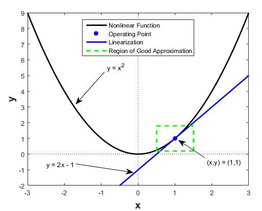
 An approximation of f(x)=x^2 at (x, f(x))

Visually, the accompanying diagram shows the tangent line of f(x) at x. At f(x+h), where h is any small positive or negative value, f(x+h) is very nearly the value of the tangent line at the point (x+h,L(x+h)).

The final equation for the linearization of a function at x=a is:

{\displaystyle y=(f(a)+f'(a)(x-a))\,}

For x=a, f(a)=f(x). The derivative of f(x) is f'(x), and the slope of f(x) at a is f'(a).
Example

To find {\sqrt {4.001}}, we can use the fact that {\sqrt {4}}=2. The linearization of f(x)={\sqrt {x}} at x=a is y={\sqrt {a}}+{\frac {1}{2{\sqrt {a}}}}(x-a), because the function f'(x)={\frac {1}{2{\sqrt {x}}}} defines the slope of the function f(x)={\sqrt {x}} at x. Substituting in a=4, the linearization at 4 is y=2+{\frac {x-4}{4}}. In this case x=4.001, so {\sqrt {4.001}} is approximately 2+{\frac {4.001-4}{4}}=2.00025. The true value is close to 2.00024998, so the linearization approximation has a relative error of less than 1 millionth of a percent.
Linearization of a multivariable function

The equation for the linearization of a function f(x,y) at a point p(a,b) is:

f(x,y)\approx f(a,b)+\left.{{\frac {{\partial f(x,y)}}{{\partial x}}}}\right|_{{a,b}}(x-a)+\left.{{\frac {{\partial f(x,y)}}{{\partial y}}}}\right|_{{a,b}}(y-b)

The general equation for the linearization of a multivariable function f(\mathbf {x} ) at a point \mathbf {p} is:

f({{\mathbf {x}}})\approx f({{\mathbf {p}}})+\left.{\nabla f}\right|_{{{\mathbf {p}}}}\cdot ({{\mathbf {x}}}-{{\mathbf {p}}})

where \mathbf {x} is the vector of variables, and \mathbf {p} is the linearization point of interest .[2]
Uses of linearization

Linearization makes it possible to use tools for studying linear systems to analyze the behavior of a nonlinear function near a given point. The linearization of a function is the first order term of its Taylor expansion around the point of interest. For a system defined by the equation

    {\frac {d{\mathbf {x}}}{dt}}={\mathbf {F}}({\mathbf {x}},t),

the linearized system can be written as

    {\frac {d{\mathbf {x}}}{dt}}\approx {\mathbf {F}}({\mathbf {x_{0}}},t)+D{\mathbf {F}}({\mathbf {x_{0}}},t)\cdot ({\mathbf {x}}-{\mathbf {x_{0}}})

where {\mathbf {x_{0}}} is the point of interest and D{\mathbf {F}}({\mathbf {x_{0}}}) is the Jacobian of {\mathbf {F}}({\mathbf {x}}) evaluated at {\mathbf {x_{0}}}.
Stability analysis

In stability analysis of autonomous systems, one can use the eigenvalues of the Jacobian matrix evaluated at a hyperbolic equilibrium point to determine the nature of that equilibrium. This is the content of linearization theorem. For time-varying systems, the linearization requires additional justification.[3]
Microeconomics

In microeconomics, decision rules may be approximated under the state-space approach to linearization.[4] Under this approach, the Euler equations of the utility maximization problem are linearized around the stationary steady state.[4] A unique solution to the resulting system of dynamic equations then is found.[4]
Optimization

In Mathematical optimization, cost functions and non-linear components within can be linearized in order to apply a linear solving method such as the Simplex algorithm. The optimized result is reached much more efficiently and is deterministic as a global optimum.
See also

    Linear stability
    Tangent stiffness matrix
    Stability derivatives
    Linearization theorem
    Taylor approximation
    Functional equation (L-function)

References

The linearization problem in complex dimension one dynamical systems at Scholarpedia
Linearization. The Johns Hopkins University. Department of Electrical and Computer Engineering
G.A. Leonov, N.V. Kuznetsov, Time-Varying Linearization and the Perron effects, International Journal of Bifurcation and Chaos, Vol. 17, No. 4, 2007, pp. 1079-1107

    Moffatt, Mike. (2008) About.com State-Space Approach Economics Glossary; Terms Beginning with S. Accessed June 19, 2008.

linearization

What Is Linearization?

Defination:

Linearization is a linear approximation of a nonlinear system that is valid in a small region around an operating point.

For example, suppose that the nonlinear function is y=x2. Linearizing this nonlinear function about the operating point x = 1, y = 1 results in a linear function y=2x−1.
Near the operating point, y=2x−1 is a good approximation to y=x2. Away from the operating point, the approximation is poor.
The next figure shows a possible region of good approximation for the linearization of y=x2. The actual region of validity depends on the nonlinear model.

Extending the concept of linearization to dynamic systems, you can write continuous-time nonlinear differential equations in this form:

˙x(t)=f(x(t),u(t),t)y(t)=g(x(t),u(t),t).

In these equations, x(t) represents the system states, u(t) represents the inputs to the system, and y(t) represents the outputs of the system.
A linearized model of this system is valid in a small region around the operating point t=t₀, x(t₀)=x₀, u(t₀)=u₀, and y(t₀)=g(x₀,u₀,t₀)=y₀.
To represent the linearized model, define new variables centered about the operating point:

δx(t)=x(t)−x0δu(t)=u(t)−u0δy(t)=y(t)−y0

The linearized model in terms of δx, δu, and δy is valid when the values of these variables are small:

δ˙x(t)=Aδx(t)+Bδu(t)δy(t)=Cδx(t)+Dδu(t)

Applications of Linearization

Linearization is useful in model analysis and control design applications.
Exact linearization of the specified nonlinear Simulink^® model produces linear state-space, transfer-function, or zero-pole-gain equations that you can use to:

• Plot the Bode response of the Simulink model.
• Evaluate loop stability margins by computing open-loop response.
• Analyze and compare plant response near different operating points.
• Design linear controller
  Classical control system analysis and design methodologies require linear, time-invariant models. Simulink Control Design™ automatically linearizes the plant when you tune your compensator. See Choosing a Control Design Approach.
• Analyze closed-loop stability.
• Measure the size of resonances in frequency response by computing closed-loop linear model for control system.
• Generate controllers with reduced sensitivity to parameter variations and modeling errors.

Linearization in Simulink Control Design

You can use Simulink Control Design to linearize continuous-time, discrete-time, or multirate Simulink models. The resulting linear time-invariant model is in state-space form.
Simulink Control Design uses a block-by-block approach to linearize models, instead of using full-model perturbation. This block-by-block approach individually linearizes each block in your Simulink model and combines the results to produce the linearization of the specified system.
The block-by-block linearization approach has several advantages to full-model numerical perturbation:

• Most Simulink blocks have preprogrammed linearization that provides Simulink Control Design an exact linearization of each block at the operating point.
• You can configure blocks to use custom linearizations without affecting your model simulation.
  See When to Specify Individual Block Linearization.
• Simulink Control Design automatically removes nonminimal states.
• Ability to specify linearization to be uncertain (requires Robust Control Toolbox™)

Model Requirements for Exact Linearization

Exact linearization supports most Simulink blocks.
However, Simulink blocks with strong discontinuities or event-based dynamics linearize (correctly) to zero or large (infinite) gain. Sources of event-based or discontinuous behavior exist in models that have Simulink Control Design requires special handling of models that include:

• Blocks from Discontinuities library
• Stateflow^® charts
• Triggered subsystems
• Pulse width modulation (PWM) signals

For most applications, the states in your Simulink model should be at steady state. Otherwise, your linear model is only valid over a small time interval.

Operating Point Impact on Linearization

Choosing the right operating point for linearization is critical for obtaining an accurate linear model. The linear model is an approximation of the nonlinear model that is valid only near the operating point at which you linearize the model.
Although you specify which Simulink blocks to linearize, all blocks in the model affect the operating point.
A nonlinear model can have two very different linear approximations when you linearize about different operating points.

The linearization result for this model is shown next, with the initial condition for the integration x₀ = 0.

This table summarizes the different linearization results for two different operating points.

Operating Point	Linearization Result
Initial Condition = 5, State x1 = 5	30/s
Initial Condition = 0, State x1 = 0	0

You can linearize your Simulink model at three different types of operating points:

• Trimmed operating point — Linearize at Trimmed Operating Point
• Simulation snapshot — Linearize at Simulation Snapshot
• Triggered simulation event — Linearize at Triggered Simulation Events